Tutorials
Defining the Geometry
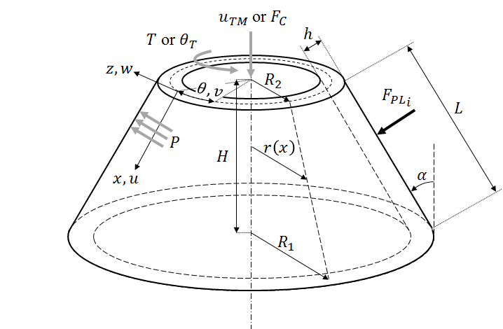
Based on the figure:
The geometry can be defined using  ,
,  and
and  , for example, or
any other combination (like
  ,
,  ,
,  ) of the geometric parameters
that will allow the complete definition of the cone / cylinder geometry.
Example:
from compmech.conecyl import ConeCyl

cc = ConeCyl()
cc.r1 = 400
cc.r2 = 200
cc.H = 200
Defining the Laminate and Material Properties
The compmech.composite module is used to calculate the laminate
properties given the stacking sequence, the thicknesses and
the material properties.
The stacking sequence is passed using a container (list or tuple)
with the orientations of each ply, from inwards to outwards:
cc.stack = [0, 0, -45, +45, -30, +30]
The ply thickness is passed using a single value when all the plies have the same thickness or using a container with the thickness of each ply:
cc.plyt = 0.125
or:
cc.plyts = [0.125, 0.125, 0.1, 0.1, 0.101, 0.101]
The material properties are given using a tuple:

where  is the elastic modulus along the direction 1 of the ply,
 the modulus along the direction 2,
  the Poisson’s ratio
and
  ,
,  ,
,  the shear modules.
Example:
cc.laminaprop = (123.55e3 , 8.708e3, 0.319, 5.695e3, 5.695e3, 5.695e3)
This will assume the same material properties for each ply. When different
properties must be used the user must supply the laminaprops container.
Example:
prop1 = (123.55e3 , 8.708e3,  0.319, 5.695e3, 5.695e3, 5.695e3)
prop2 = (100.2e3 , 4.2e3,  0.2, 5.1e3, 5.1e3, 5.1e3)
prop3 = (100.2e3 , 4.2e3,  0.2, 5.1e3, 5.1e3, 5.1e3)
cc.laminaprops = [prop1, prop1, prop2, prop2, prop3, prop3]
Linear Static Analysis
The static analysis is executed using the
compmech.conecyl.ConeCyl.static() method. The following example will
give an overview of the main steps needed for a linear static analysis.
Defining the geometry:
>>> cc.laminaprop = (123.55e3 , 8.708e3,  0.319, 5.695e3, 5.695e3, 5.695e3)
>>> cc.stack = [0, 0, 19, -19, 37, -37, 45, -45, 51, -51]
>>> cc.r2 = 250.
>>> cc.H = 510.
>>> cc.plyt = 0.125
>>> cc.alphadeg = 30.
Defining the model and boundary conditions:
>>> cc.model = 'fsdt_donnell_bc1'
>>> cc.bc = 'cc1'
Defining if the analysis is displacement or load controlled by changing
the boolean parameters pd (prescribed displacement):
prescribed displacement for compression:
cc.pdCprescribed displacement for torsion:
cc.pdTprescribed load asymmetry
cc.pdLA
Applying the axial compression, pressure, torsion and the single-perturbation loads:
>>> cc.Fc = 10000.
>>> cc.T = 100000.
>>> cc.P = -0.01
>>> cc.add_SPL(10.)
>>> cc.add_SPL(4.)
Defining the number of terms in the approximation functions:
>>> cc.m1 = 80
>>> cc.m2 = 40
>>> cc.n2 = 40
Running the analysis:
>>> cc.static()
The results are stored in the cs list, and for a linear static analysis
only one entry exists. Plotting the results:
>>> cc.plot(cc.cs[0], vec='w')
Static Analysis
where NLgeom is a flag telling whether or not a geometric non-linear
analysis is to be performed.
The solution is stored in the cs attribute, which consists of a list
of 1-D np.ndarray objects. For a linear analysis this list will contain
only one entry while for a non-linear analysis it will contain one entry
for each iteration needed up to the convergence or up to the termination
criterion. To access the last result:
solution = cc.cs[-1]
The displacement field can be plotted, for example:
cc.plot(solution, vec='w', filename='my_output.png')
Non-Linear Analysis
Using NLgeom=True in a static analysis will run a geometrically
non-linear analysis. Many attributes of the ConeCyl object
are used to control the non-linear analysis (see
ConeCyl.static()).
The converged increments used along the non-linear analysis are stored
in the increments attribute and the corresponding solutions
stored in the cs attribute (a list of 1-D np.ndarray objects).

